Microsoft Excel 2007

Microsoft Excel Window

 

 Menu 

 

AutoSum 

The following illustrates AutoSum:

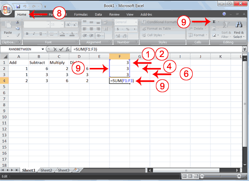
1. Go to cell F1.
2. Type 3.
3. Press Enter. Excel moves down one cell.
4. Type 3.
5. Press Enter. Excel moves down one cell.
6. Type 3.
7. Press Enter. Excel moves down one cell to cell F4.
8. Choose the Home tab.
9. Click the AutoSum button in the Editing group. Excel selects cells F1 through F3 and enters a formula in cell F4.

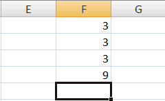
10. Press Enter. Excel adds cells F1 through F3 and displays the result in cell F4.

 

Create Borders 

 

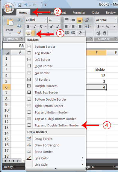
2. Choose the Home tab.
3. Click the down arrow next to the Borders button . A menu appears.
4. Click Top and Double Bottom Border. Excel adds the border you chose to the selected cells.

Add Background Color

 

 

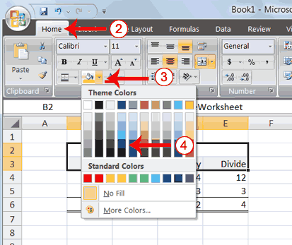
2. Choose the Home tab.
3. Click the down arrow next to the Fill Color button .
4. Click the color dark blue. Excel places a dark blue background in the cells you selected.

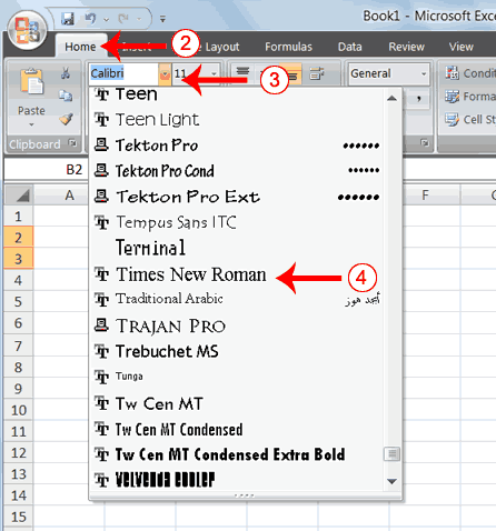
Change the Font

 

1. Select cells B2 to E3.

1. Choose the Home tab.
2. Click the down arrow next to the Font box. A list of fonts appears. As you scroll down the list of fonts, Excel provides a preview of the font in the cell you selected.
3. Find and click Times New Roman in the Font box. Note: If Times New Roman is your default font, click another font. Excel changes the font in the selected cells.

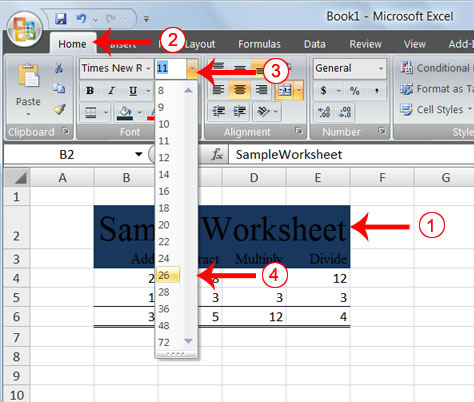
Change the Font Size

 

1. Select cell B2.
2. Choose the Home tab.
3. Click the down arrow next to the Font Size box. A list of font sizes appears. As you scroll up or down the list of font sizes, Excel provides a preview of the font size in the cell you selected.
4. Click 26. Excel changes the font size in cell B2 to 26.

 

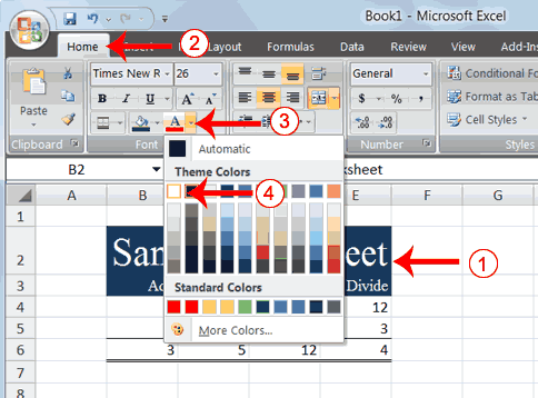
 Change the Font Color

 

1. Select cells B2 to E3.
2. Choose the Home tab.
3. Click the down arrow next to the Font Color button .
4. Click on the color white. Your font color changes to white.

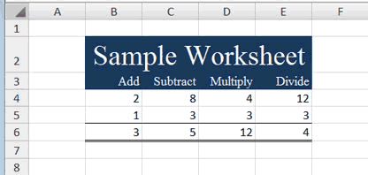
Your worksheet should look like the one shown here.

 

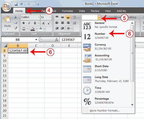
Format Numbers

4. Choose the Home tab.
5. Click the down arrow next to the Number Format box. A menu appears.
6. Click Number. Excel adds two decimal places to the number you typed.
7.  
8.  
9.  

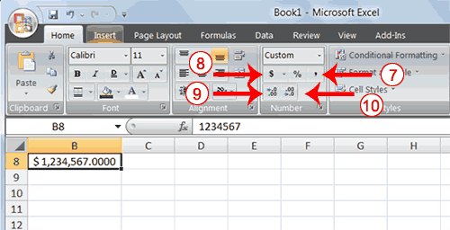
7. Click the Comma Style button . Excel separates thousands with a comma.
8. Click the Accounting Number Format button . Excel adds a dollar sign to your number.
9. Click twice on the Increase Decimal button to change the number format to four decimal places.
10. Click the Decrease Decimal button if you wish to decrease the number of decimal places.

 

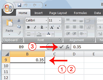
Change a decimal to a percent.

 

1. Move to cell B9.
2. Type .35 (note the decimal point).
3. Click the check mark on the formula bar.

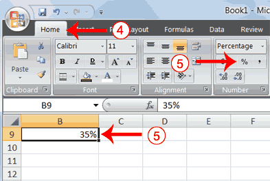
4. Choose the Home tab.
5. Click the Percent Style button . Excel turns the decimal to a percent.

 

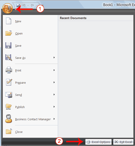
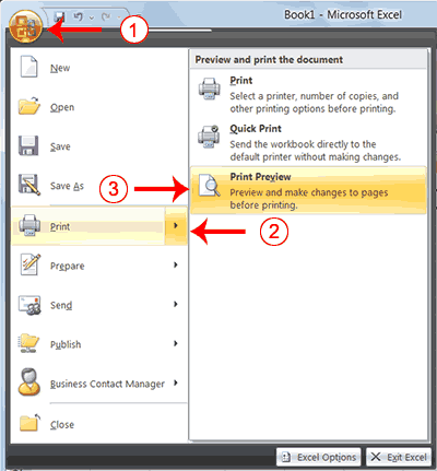
Print Preview

 

1. Click the Office button. A menu appears.
2. Highlight Print. The Preview and Print The Document pane appears.
3. Click Print Preview. The Print Preview window appears, with your document in the center.

 

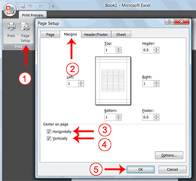
Center Your Document

 

1. Click the Page Setup button in the Print group. The Page Setup dialog box appears.
2. Choose the Margins tab.
3. Click the Horizontally check box. Excel centers your data horizontally.
4. Click the Vertically check box. Excel centers your data vertically.
5. Click OK. The Page Setup dialog box closes.

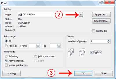
Print

1. Click the Print button. The Print dialog box appears.
2. Click the down arrow next to the name field and select the printer to which you want to print.
3. Click OK. Excel sends your worksheet to the printer. 

Create a Chart

 

.

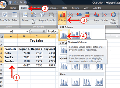
1. Select cells A3 to D6. You must select all the cells containing the data you want in your chart. You should also include the data labels.
2. Choose the Insert tab.
3. Click the Column button in the Charts group. A list of column chart sub-types types appears.
4. Click the Clustered Column chart sub-type. Excel creates a Clustered Column chart and the Chart Tools context tabs appear.

 

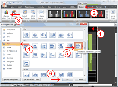
Change the Chart Type

 

1. Click your chart. The Chart Tools become available.
2. Choose the Design tab.
3. Click Change Chart Type in the Type group. The Chart Type dialog box appears.
4. Click Bar.
5. Click Clustered Horizontal Cylinder.
6. Click OK. Excel changes your chart type.